High-quality Surface Reconstruction using Gaussian Surfels

本质上这篇文章也是一个 2DGS

项目地址

SIGGRAPH 2024

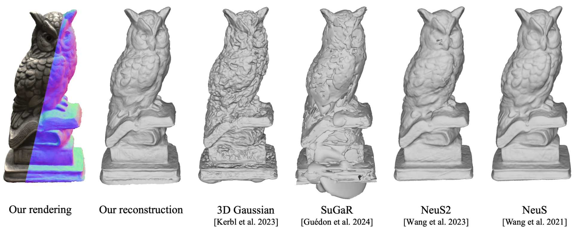
Fig. 1: Overview

Abstract

本文提出了一种新颖的基于点的表示法——高斯表面元素 (Gaussian Surfels)，将 3D 高斯点的灵活优化优势和表面对齐特性结合起来。这是通过直接将 3D 高斯点 z 轴的 scale 设为 0 来实现的，从而有效地将原始的 3D 椭圆体扁平化为 2D 椭圆。这样的设计为优化器提供了明确的指导。通过将局部 z 轴作为法线方向，大大提高了优化的稳定性和表面对齐度。虽然在这种情况下，根据协方差矩阵计算出的本地 z 轴导数为零，但本文设计了一种自监督法线深度一致性损失来解决这个问题。为了提高重建质量，还加入了单目法线先验和前景 mask，以减轻与高光和背景相关的问题。本文提出了一种体积切割方法来汇总高斯表面的信息，从而去除 alpha 混合生成的深度图中的错误点。最后，将经过筛选的泊松重建方法应用于融合深度图，以提取表面网格。实验结果表明，与最先进的神经体积渲染和基于点的渲染方法相比，本文的方法在表面重建方面表现出了卓越的性能。

Introduction

作者认为 3DGS 在重建表面方面存在缺陷，主要是由三个方面导致的：

1. 因为 3D 高斯基元是个椭球，没法与表面对齐
2. 椭球的法向量没办法确定。
3. alpha 混合过程可能会给重建的表面边缘带来偏差，因为在混合的过程中可能会混合一些边缘之外的高斯基元。

总结来说都是因为 3D 高斯基元是个椭球导致没法完美贴合在表面上

本文的贡献为：

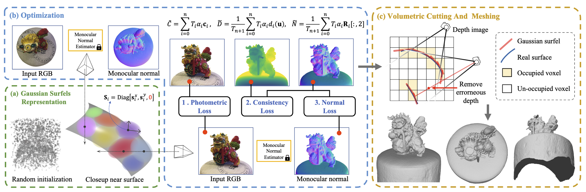
• 提出了一种新颖的基于点的表示法——高斯表面元素 (Gaussian Surfels)，以解决 3DGS 固有的法线模糊，并实现与实际表面的紧密对齐。结合体积切割方法，表面重建的质量得到了显著提高。
• 提出了一种自监督法线深度一致性正则项以及光度损失正则项，指导高斯表面以密切贴合物体表面的方式移动和旋转。将单目估计法线作为先验值，以解决镜面反射区域的形状亮度模糊问题。
• 与最先进的基于神经体积和点的渲染方法相比，本文的方法在重建质量和训练速度之间实现了良好的平衡。

Method

Fig. 2: Pipeline

如图 2 所示，本文以一组 RGB 图片作为输入，$\mathbf{I}_k$ 表示第 $k$ 张图片。以一组由各向异性的椭圆高斯核所表示的 Gaussian Surfels 作为输出。通过最小化渲染图片和 GT 之间的光度损失来优化 Gaussian Surfels，为了使优化可控，还使用了正则化损失来强制表面平滑和深度法线一致性。最后用屏蔽泊松表面重建算法 (Screened Poisson Surface Reconstruction) 来提取高质量的 mesh，在提取 mesh 之前，用体积切割 (volumetric cutting) 来减少因表面边界像素的 alpha 混合而产生的错误深度值。

Gaussian Surfels

Gaussian Surfels 由一组无结构化的高斯核 $\left\{\mathbf{x}_i, \mathbf{r}_i, \mathbf{s}_i, o_i, C_i\right\}_{i \in \mathcal{P}}$ 组成，因此 3D 高斯的分布可以表示为：

$$G\left(\mathbf{x} ; \mathbf{x}_i, \Sigma_i\right)=\exp \left\{-0.5\left(\mathbf{x}-\mathbf{x}_i\right)^{\top} \Sigma_i^{-1}\left(\mathbf{x}-\mathbf{x}_i\right)\right\} \tag{1}$$

• $\mathbf{x}_i\in\R^3$ 表示高斯核的中心位置
• $\mathbf{r}_i\in\R^4$ 表示由四元数表示的高斯核的旋转
• $\mathbf{s}_i\in\R^e$ 表示高斯核两个轴的缩放因子
• $o_i\in\R$ 表示高斯核的不透明度
• $C_i\in\R^k$ 表示高斯核的球谐函数系数
• $\Sigma_i$ 是协方差矩阵

高斯核和高斯基元是同一个意思

将 $\mathbf{s}_i=[\mathbf{s}_i^x,\mathbf{s}_i^y,0]^\top$ 来压扁一个 3D 高斯，因此对应的 $\Sigma_i$ 变为：

$$\Sigma_i=\mathbf{R}\left(\mathbf{r}_i\right) \mathbf{S}_i \mathbf{~S}_i^{\top} \mathbf{R}\left(\mathbf{r}_i\right)^{\top}=\mathbf{R}\left(\mathbf{r}_i\right) \operatorname{Diag}\left[\left(\mathbf{s}_i^x\right)^2,\left(\mathbf{~s}_i^y\right)^2, 0\right] \mathbf{R}\left(\mathbf{r}_i\right)^{\top} \tag{2}$$

• $\mathrm{Diag}[\cdot]$ 表示对角矩阵

每个高斯核的法向量可以直接表示为 $\mathbf{n}_i=\mathbf{R}(\mathbf{r}_i)[:,2]$，通过优化每个椭圆的朝向来使 Gaussian Surfels 和真实的表面对齐。

可微 Gaussian splatting 和 3DGS 基本上没区别。每个像素点的深度 $\tilde{D}$ 和法向量 $\tilde{N}$ 也可以通过 Gaussian splatting 和 alpha 混合计算出：

$$\tilde{N}=\frac{1}{1-T_{n+1}} \sum_{i=0}^n T_i \alpha_i \mathbf{R}_i[:, 2], \quad \tilde{D}=\frac{1}{1-T_{n+1}} \sum_{i=0}^n T_i \alpha_i d_i(\mathbf{u}) \tag{3}$$

对于深度渲染，直接用高斯核的中心位置来计算深度是不正确的，因为这样忽视了椭圆的倾斜。如图 3 所示，第一行直接用椭圆的中心位置来估计深度，这样会产生误差；第二行用光线和椭圆的交点作为深度。

Fig. 3: The first row: the intersection of a ray with a 3D Gaussian point is challenging to calculate precisely. As a result, approximate the depth of intersection with the depth of the Gaussian's center point, which can introduce errors. The second row: the intersection of a ray with our Gaussian surfel can be calculated precisely, as well as its depth.

在 splatting 的过程中，通过计算穿过像素 $\mathbf{u}$ 的光线和高斯核 $i$ 的交点，这个过程可以通过局部泰勒展开简化为：

$$d_i(\mathbf{u})=d_i\left(\mathbf{u}_i\right)+\left(\mathbf{W}_k \mathbf{R}_i\right)[2,:] \mathbf{J}_{p r}^{-1}\left(\mathbf{u}-\mathbf{u}_i\right) \tag{4}$$

• $\mathbf{J}^{-1}_{pr}$ 表示将屏幕空间中的像素点反投影到 Gaussian Surfels 的切平面空间的雅可比矩阵
• $(\mathbf{W}_k\mathbf{R}_i)$ 表示将 Gaussian Surfels 的旋转矩阵变换到相机空间

Optimization

Photometric loss. 光度损失和 3DGS 中一样：

$$\mathcal{L}_\mathrm{p}=0.8\cdot L_1(\tilde{\mathbf{I}},\mathbf{I})+0.2\cdot L_{DSSIM}\cdot(\tilde{\mathbf{I}},\mathbf{I}) \tag{5}$$

• $\tilde{\mathbf{I}}, \mathbf{I}$ 分别表示渲染出来的图像和 GT

Depth-normal consistency loss. 这个正则项用来约束渲染深度和渲染法向量之间的一致性：

$$\mathcal{L}_c=1-\tilde{\mathbf{N}}\cdot N(V(\tilde{\mathbf{D}})) \tag{6}$$

• $\tilde{\mathbf{N}},\tilde{\mathbf{D}}$ 分别表示渲染深度和渲染法向量
• $V(\cdot)$ 将每个像素的深度映射回 3D 点
• $N(\cdot)$ 通过相邻点法向量的叉乘计算当前点的法向量

这个正则项在本文的优化过程中起着至关重要的作用，尤其是在解决每个 Gaussian Surfels 的梯度消失问题时。

Normal-prior loss. 在高光的区域，光度损失可能会导致错误的表面，因此用预测的法向量图作为先验，来提高优化的稳定性：

$$\mathcal{L}_{\mathrm{n}}=0.04 \cdot(1-\tilde{\mathbf{N}} \cdot \hat{\mathbf{N}})+0.005 \cdot L_1(\nabla \tilde{\mathbf{N}}, \mathbf{0}) \tag{7}$$

• $\hat{\mathbf{N}}$ 表示预测出来的法向量图
• $\nabla \tilde{\mathbf{N}}$ 表示渲染法向量的梯度，对表面的曲率进行正则化

Opacity loss. 不透明度损失来约束每个高斯核的不透明度尽量要么为 0 要么为 1：

$$\mathcal{L}_o=\exp(-(o_i-0.5)^2/0.05) \tag{8}$$

• $o_i$ 是经过 sigmoid 后得到的不透明度

最终的 loss 为：

$$\mathcal{L}=\mathcal{L}_{\mathrm{p}}+\mathcal{L}_{\mathrm{n}}+\lambda_{\mathrm{o}} \mathcal{L}_{\mathrm{o}}+\lambda_{\mathrm{c}} \mathcal{L}_{\mathrm{c}}+\lambda_{\mathrm{m}} \mathcal{L}_{\mathrm{m}} \tag{9}$$

• $\mathcal{L}_m$ 为渲染 alpha 图和分割 mask 之间的二元交叉熵损失

Gaussian Point Cutting and Meshing

通过融合渲染的深度图和法线图，然后应用屏蔽泊松表面重建算法 (树深度为 10) 来获得最终的 mesh。

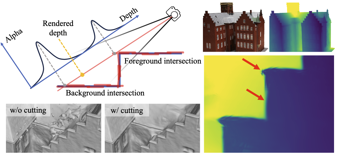
但是如图 4 所示，如果椭圆超出了真正的表面边界，且相关权重无法快速衰减为零，则背景表面的渲染深度将受到前景高斯核 alpha 值的影响，导致深度错误。由于 Gaussian Surfels 的复杂分布，很难通过丢弃远离中位数或 alpha 加权平均值的 surfels 来去除每条射线上的异常值。因此根据每个 Gaussian Surfels 的累积的 alpha 值实施体积切割。

Fig. 4: An example of error in the rendered depth

Volumetric cutting. 这样做的目的是将那些远离 Gaussian Surfels 的体素标记为未占用体素，即从 grid 中删除这些体素。因此，图 4 中红色的错误 3D 点可以被删除，因为它位于未被占用的体素内部。具体来说，首先在 bounding box 内构建 $512^3$ 个体素网格。然后，遍历所有高斯椭圆，计算它们与周围体素的交点，并累积相应体素的加权不透明度 $G(\mathbf{x},\mathbf{x}_i,\Sigma_i)\cdot o_i$。为了降低计算成本，使用体素中心的加权不透明度来近似交叉区域内的高斯权重和不透明度。如果一个体素的累积加权不透明度较低，在实验中低于 $\lambda=1$，表明与前景或背景表面的距离较大，就会剪除这些体素以及其中根据深度计算出的 3D 点。

Reference

[1]High-quality Surface Reconstruction using Gaussian Surfels